Deterministic landslide hazard analysis in GIS.
A case study from Manizales (Colombia)
C.J. van Westen and M.T.J. Terlien
ITC, PO Box 6, 7500 AA Enschede, The Netherlands.
Published in: Earth Surface Processes and Landforms, Vol.21, 853-868 (1996)
![]()
ABSTRACT
A one-dimensional deterministic slope stability model (infinite slope model) was used to calculate average safety factors and failure probabilities for the city of Manizales, in central Colombia. An engineering geological data base has been created on the basis of a series of parameter maps, using logic reasoning in GIS. A two dimensional hydrological model was applied to estimate groundwater levels in relation to rainfall events. A simple method for the calculation of horizontal seismic acceleration was used for different earthquake events. To calculate average safety factors a number of scenarios were developed, by combining the effects of groundwater and seismic acceleration with different return periods. A simple method for error propagation was used to calculate the variance of the safety factor, and the probability that it will be less than 1, for each pixel, within a time period of 20 years. The highest probability value of the various scenarios was selected for each pixel, and a final hazard map for translational landslides was constructed.
![]()
1. Introduction
A large amount of research on landslide hazard zonation has been done over the last 30 years as the consequence of an urgent demand for slope instability hazard information for planning purposes. Overviews of the various slope instability hazard zonation techniques can be found in Hansen (1984), and Varnes (1984). Initially the investigations were oriented mainly towards problem solving at the scale of site investigation and development of deterministic models. A wide variety of deterministic slope stability methods is now available to the engineer. Reviews of these can be found in, for example, Graham (1984), and Anderson and Richards (1987). The application of deterministic models for the zonation of hazard in larger areas, however, never has had a large development, due to the regional variability of geotechnical variables such as cohesion, angle of internal friction, thickness of layers, or depth to groundwater. Furthermore, the calculation of safety factors over larger areas involves an extremely large number of calculations, which could not be executed without the use of Geographic Information Systems.
Despite of these problems, deterministic models are increasingly used in hazard analysis over larger areas. Currently, only the use of deterministic models will result is real hazard maps, according to Varnes's definition: "Natural hazard means the probability of occurrence of a potentially damaging phenomenon within a specified period of time and within a given area" (Varnes, 1984). Deterministic models, combined with the magnitude/frequency information of triggering events (rainfall, earthquakes), make it possible to derive at a probability of failure, which can then be used in risk studies or in the design of engineering structures.
Deterministic slope stability models are only applicable in landslide hazard zonation when the geomorphological and geological conditions are fairly homogeneous over the entire study area and the landslide types are simple. In more heterogenous areas they may lead to an undesirable generalization.
For the application of GIS in deterministic modelling one-, two- or three-dimensional approaches can be followed. The most complex calculation procedure, using three-dimensional slope stability programs, requires the sampling of data at predefined grid-points, and exportation of these data to an external three-dimensional slope stability model. This is only applicable for very small areas, where a large amount of data is available, and is therefore not used in regional slope stability zonation.
Also the use of two-dimensional slope stability programs in a GIS environment is very seldomly used (Van Asch et al. 1993). This method requires the selection of a number of profiles from a DTM and other parameter maps. The resulting data are exported to external slope stability models. The main advantage of this approach is that external existing models can be used without losing time in programming the model algorithms in a GIS. The disadvantages of model calculations outside GIS are data conversion, and the use of the results of the model calculations in the construction of a landslide hazard map. The safety factors, calculated along the profiles, should be interpolated, or linked to geomorphological units, which may be very difficult.
The most suitable method for the use of deterministic models in a GIS environment is the one-dimensional infinite slope modelling (Ward et al., 1982; Brass et al., 1989; Murphy and Vita-Finzi, 1991). It is the only model which calculates slope instability on a pixel basis, and is therefore very suitable to be used in a raster GIS.
The one-dimensional infinite-slope model describes slope stability in the simplest form. It is only applicable for the calculation of shallow translational slides. Slope stability is calculated for the pixels on a map, using information combined from several input maps, such as slope angle, soil depth, soil strength, and depth to groundwater. Calculations for each individual pixel will result in safety factor values, which can be used to create a hazard map.
The basic formula for the infinite slope model is (after Graham, 1984):

where:
F = safety factor, c´ = effective cohesion (Pa), z = depth of failure surface below the terrain surface (m), which is equal to the thickness of ashes as we are assuming a failure surface at the base of the ashes,
g = unit weight of soil (N/m3), b = terrain surface inclination (°), r = bulk density in (kg/m3), ah = peak horizontal acceleration in rock (m/s2), and N = amplification of seismic acceleration in soil material (dimensionless), gw = unit weight of water (N/m3), m = groundwater/soil thickness ratio zw/z (dimensionless), zw = height of water table above failure surface (m), and n´ = effective angle of shearing resistance (°).For calculation purposes equation [1] was divided into two parts [2], later indicated as B1 and B2:

![]()
2. The study area
In the framework of two international research projects, financed by the European Union, UNESCO and the Netherlands government, a methodology was developed for the use of GIS in landslide hazard zonation (Van Westen et al, 1993). The methods were tested in a study area in Central Colombia, surrounding the city of Manizales (see figure 1). Manizales (300.000 inhabitants) is located at an altitude of 2000 m on the western flank of the Cordillera Central, near the Nevado del Ruiz volcano. Due to its unfavourable topographic location, large parts of the city are built on steep slopes, which are mostly modified by cuts and (hydraulic) fills to provide adequate terrain for housing. Manizales has suffered strongly from landslide problems. The landslides are a result of the geological and geomorphological setting of the area, the wet climate, and the fact that the area is located in a seismically active region. The geology of the area consists of meta-sedimentary schists from the Quebradagrande formation of Cretaceous age covered by fluvio-volcanic materials from Tertiary age (Manizales and Casabianca formations, consisting of debris flow material, pyroclastic flows, alluvial materials and intercalated ashes) with different degrees of weathering. Nearly the entire area is mantled by volcanic ashes of Quaternary age (Naranjo and Rios, 1989). The thickness of the ashes varies from 11 m on the flat hilltops to 1 m or less on very steep slopes. The ash deposits contain layers with textures ranging from very fine (< 63mm) to very coarse (> 5000 mm) (Van Westen et al, 1993). These changes in texture cause perched watertables in the ashes, which can trigger soilslips, soil avalanches, and translational slides. Most translational slides are caused by high groundwater levels in the volcanic ashes overlying impermeable residual soil from schists of the Quebradagrande formation.
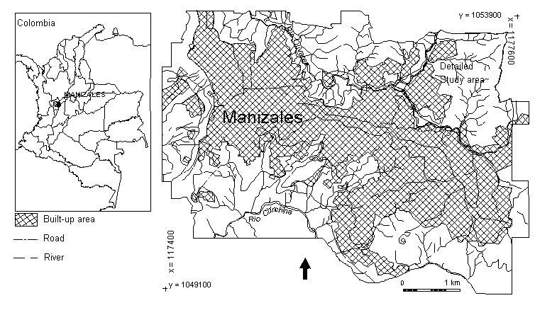
Figure 1: Location of the study area in Colombia
![]()
3. The input data
To evaluate the stability of the entire city of Manizales on a general scale (1:10.000) the following steps were taken:
1. Construction of an engineering geological data base;
2. Groundwater modelling;
3. Calculation of maximum horizontal seismic accelerations;
4. Slope stability calculations using different scenarios for groundwater levels and seismic accelerations;
3.1 Engineering geological data base
Due to the heterogeneous nature of the superficial materials in Manizales, its rugged topography and the small amount of drillhole information available, the engineering geological data base could not be obtained from interpolation of material depths, derived from drillholes and outcrops. Therefore, another method was developed based on the use of logic reasoning in GIS. With this method the spatial distribution of the various materials could be deduced from a very detailed geomorphological map, three landslide distribution maps from different periods, a geological map, and two DTM's from different dates with accompanying slope maps. Combining the different maps using conditional statements in GIS made it possible to produce the engineering geological data base. This data base describes the materials in three dimensions, showing both the spatial distribution of 4 basic materials layers, and their thicknesses. As we are working with a 2-Dimensional GIS system (ILWIS) this was done by separating the spatial information from the thickness information (see figure 2). This way 8 different maps were used which provide the soil profile for any pixel if they are read simultaneously using a pixel-information program. The maps show the spatial distribution of the four layers with the same material codes and can be linked with tables containing geotechnical properties derived from laboratory tests, and field measurements. The procedure is explained in detail in Van Westen et al (1993, in press).
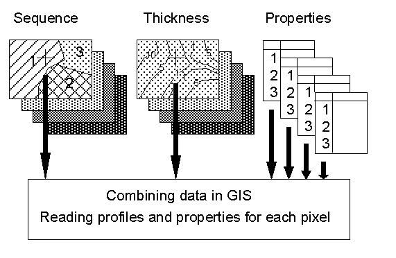
Figure 2: Simplified structure of the engineering geological data base for Manizales. Separate maps are made for the spatial distribution of materials (Sequence), and for the thickness of materials. Profiles can be obtained by reading all maps simultaneously in a GIS, and combining them with geotechnical properties from tables.
3.2 Groundwater simulations
In the case of deterministic landslide hazard zonation distributed hydrological and slope stability programmes are used to calculate the spatial distribution of piezometer levels and pore pressures. Also for hydrological models a choice can be made between one-, two- and three-dimensional models (Okimura and Kawatani, 1986; Terlien et al, in press).
For the groundwater modelling a simple 2-dimensional model was used (Van Asch et al, 1992). This computer model calculates ground water levels on a daily basis in layers with different hydrological properties. As we were interested in the contact between volcanic ash materials and residual soils we used a two-layer model, under a large number of different profiles, with respect to slope angle, slope length, ash-thickness, and saturated conductivity. The maximum groundwater levels for each of these profiles were calculated for a 20 year period and used in the construction of magnitude-frequency curves. Then the profiles were linked to the maps using the engineering geological data base and the topographic information, and groundwater maps were derived for different return periods (Van Westen et al, 1993).
3.3 Seismic acceleration
In order to be able to calculate seismic acceleration, information should be available on the magnitude, frequency, and distance of seismic events, the material sequences, geotechnical data, groundwater levels, and topographic conditions. Unfortunately, no seismic data from accelerographs were available for the study area.
Many equations have been suggested to calculate peak ground acceleration for hard rock in relation to the magnitude and focal distance of a seismic event (Hays, 1980). These equations are applicable only in those areas where they were developed. Donovan (1973) used worldwide data to derive a general equation:
![]()
where: ah = peak horizontal acceleration for hard rock (m/s2), M = magnitude (Richter scale), and R = hypocentre distance (km).
The value of 0.24 m/s2, derived by this method for the 1979 earthquake (magnitude 6.3, distance to hypocenter 130 km) was approximately twice as high as one the scarce values for acceleration at the surface, reported in Manizales (Geotecnia, 1980). This means that there is a strong amplification of the seismic waves due to topographic and geotechnical conditions.
A very simple estimation of the amplification of the seismic wave due to different materials can be obtained, derived from the work of Medvedev (1965):
![]()
where: N = amplification of acceleration (dimensionless), v0 = seismic wave velocity of the material below the contact (m/s), r0 = bulk density of the material below the contact (kg/m3), v1 = seismic wave velocity of the material above the contact (m/s), r1 = bulk density of the material above the contact (kg/m3), and cf = correction factor for the depth of the phreatic water level. The acceleration values at the surface can be calculated by multiplying N (equation [4]) by the maximum acceleration in hard rock, derived from equation [3].
In order to be able to calculate return periods for acceleration values, return periods are first selected for magnitudes of earthquakes. A record of 331 earthquakes occurring within the area between 4.5-6.0° north latitude and 74.5-76.5° west longitude was collected for the period 1922 to 1979 from the literature (James, 1986; Valencia, 1988; Page, 1986). On the basis of this data, the following relationship between magnitude and return period was calculated (Valencia, 1988):
![]()
where: M = magnitude on the Richter scale, and RY = return period in years.
To calculate maximum acceleration in hard rock for seismic events one must assume a distance to the hypocentre. A relatively short distance of 112 km was used ( 50 km to epicentre and 100 km depth of hypocentre), which is equal to the distance to the hypocentre of the 1962 earthquake. The resulting acceleration values for several events are given in table 1. The data used to calculate amplification for a standard profile in the Manizales area is given in table 2 (after Geotecnia, 1980).
|
Magnitude (Richter) |
Return period in years |
Peak acceleration in rock: ah (m/s2) |
|
7.5 |
32 |
0.578 |
|
6.9 |
20 |
0.408 |
|
6.5 |
15 |
0.324 |
|
6.0 |
10 |
0.242 |
|
5.5 |
7 |
0.214 |
Table 1: Some values for peak acceleration at the rockhead (ah), calculated for different earthquakes. Assumed distance to hypocenter is 112 km.
|
Material |
Seismic velocity v (m/s) |
Bulk density r (kg/m3) |
|
Fill |
0.30 |
1300 |
|
Volcanic ash |
0.38 |
1400 |
|
Manizales Formation |
2.14 |
2000 |
|
Quebradagrande Formation |
3.2 |
2600 |
Table 2: Geotechnical properties of the main material types in the Manizales area, used to calculate seismic amplification (after Geotecnia, 1980).
Based on the values in table 2 the amplification for different sequences of materials can be calculated from equation [4]. For example, a sequence of fill-ash-Manizales formation-Quebradagrande formation will result in an amplification value of 0.48 + 1.51 + 0.23 = 2.22. A correction factor of 1 was used for groundwater occurring within 1 m below the surface and an amplification value of 0.5 for groundwater occurring between 1 and 4 m below the surface (James, 1986).
With the data from tables 1 and 2 and with the engineering geological data base, acceleration values can be calculated for each pixel for a given seismic event.
![]()
4. Evaluating possible failure conditions
As mentioned in the introductory section, the use of even a very simple slope stability model is only feasible in relatively homogenous terrain. Since the material thicknesses are the most crucial uncertainty in the analysis, an evaluation was made of the critical depth of translational landslides, by solving equation [2] for the case F = 1. Based on this equation a number of different scenarios were evaluated.
In figure 3 some of the values for the relationship between the depth of the sliding plane and the surface slope angle, derived from a set of translational landslides, that were measured in the Manizales area, are plotted together with some critical depth lines for extreme conditions of c´ and m. It is clear from this figure that landslides occur over a very wide range of soil thicknesses and surface slope angles. Slope angles are generally larger than 25°, and soil thicknesses range from 1 and 10 m. With the exception of one, all points are located between the maximum possible limits of cohesion and groundwater/soil depth relations. The conditions under which failure occurs are very different, and the use of one value for cohesion or groundwater/soil depth relation will lead to a simplification. The straight line displays the relationship between ash thickness and slope angle which was used to make an ash-thickness map.
A calculation was made to estimate the number of pixels in the map that would have safety factors lower than 1 when the different conditions mentioned above would be applied (table 3). From this table it can be observed that groundwater/soil depth ratios of 0.5 and 1 lead to an extremely large percentage of pixels with a safety factor less than 1. This situation is, of course, very unlikely. Groundwater/soil depth ratios are not constant for different ash thicknesses. With small ash thicknesses this ratio may be as high as 1, and for thick ash it is seldom higher than 0.3. The influence of cohesion can also be evaluated from table 3. In the case of a cohesion of 5 KPa and an earthquake acceleration an unrealistically high percentage of the area is predicted to fail, even under dry conditions.
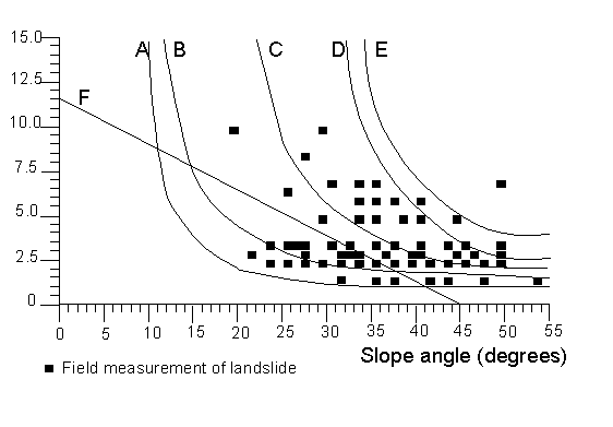
Figure 3: Values for the relationship between sliding plane depth and surface slope angle, measured for translational landslides in Manizales (black dots), plotted together with critical depth/slope angle relations calculated for some extreme values of cohesion (c´) and groundwater/soil depth ratio (m = zw/z). A: c´= 5 KPa, m =1, B: c´= 10 KPa, m= 1, C: c´= 10 KPa, m= 0.5, D: c´= 10 KPa, m=0, E: c´= 15 KPa, m= 0, F: the relationship between ash thickness and slope angle which was used to make the ash thickness map.
When the results from table 3 are compared with figure 3 it is clear that the map includes many other combinations of slope angle and ash or fill thickness than those predicted with the model (straight line in figure 3). The reason for the deviation is the occurrence of fill material on top of the ash. Fill thickness was calculated as the difference in DTMs between 1949 and 1989. For those pixels with a fill thickness value that value was added to the thickness value coming from the straight line. For those pixels where the terrain had been excavated, the excavation depth value was subtracted from the depth obtained from the straight line. The lower part of table 3 displays the results of calculations performed on the fill materials. It appears that at 3700 pixels (1% of the map) the slopes always will fail, even in dry conditions and with high values for cohesion. This result must be due to errors in the DTMs and the slope maps.
|
Effective cohesion c´ (KPa) |
Seismic acceleration at surface a (m/s2) |
Relation groundwater soildepth m (-) |
Percentage of map with safety factor <1 |
|
5 5 5 5 5 5 5 5 5 10 10 10 10 10 10 10 10 10 15 15 15 15 15 15 15 15 15 |
0 0 0 0.6 0.6 0.6 1.2 1.2 1.2 0 0 0 0.6 0.6 0.6 1.2 1.2 1.2 0 0 0 0.6 0.6 0.6 1.2 1.2 1.2 |
0 0.5 1 0 0.5 1 0 0.5 1 0 0.5 1 0 0.5 1 0 0.5 1 0 0.5 1 0 0.5 1 0 0.5 1 |
3 22 58 4 33 72 17 45 88 2 5 45 3 19 60 4 35 76 1 3 28 2 3 5 3 7 62 |
|
Calculation for pixels with fill only |
|||
|
c ´ (KPa) |
a (m/s2) |
m (-) |
Percentage of map F<1 |
|
5 10 15 |
0 0 0 |
0 0 0 |
2 1 1 |
Table 3: Percentage of pixels in the study area with ash and/or fill material failing under different conditions of c´ (effective cohesion), a (seismic acceleration), and m (relation groundwater/soil depth). The lower section shows the error due to the presence of fill material.
Before the safety-factor maps were calculated it was considered important to remove from the data set the impossible combinations, caused by errors in the input data. The material maps contain obviously many combinations of soil thickness and slope angle, which are caused by errors in calculating fill thickness from DTMs. All points falling to the right of the curve showing critical depth for a cohesion of 15 KPa under dry conditions and without earthquake acceleration (line E in figure 3) were displaced horizontally until they reached line E. This means that with any small increase of groundwater level or earthquake acceleration the terrain at these pixels will fail.
![]()
4. Factor-of-safety maps
Factor of safety maps were calculated, using equation [2], for a number of scenarios, with different magnitudes of rainfall related groundwater levels, and seismic accelerations.
Six scenarios were calculated:
1. Dry condition, without earthquake.
2. Groundwater with return period of 20 years, without earthquake.
3. Completely saturated condition, without earthquake.
4. Dry condition, with an earthquake of 6.9 Magnitude, with a return period of 20 years and occurring at a hypocentral distance of 112 km.
5. Groundwater with return period of 0.16 years (occurring 2 months per year), and an earthquake with a return period of 20 years.
6. Groundwater with return period of 20 years, and an earthquake with a return period of 20 years.
The parameters used in equation [2] for the six scenarios are presented in table 4. As can be seen from this table, some of the parameters are entered as values, and other are maps (shown in bold), related to different return periods.
|
Parameters in equation [2] |
SCENARIOS |
|||||
|
1 |
2 |
3 |
4 |
5 |
6 |
|
c ´ (Pa)z (m) g (N/m3)r (kg/m3)a (m/s2) N (-) Tan n´ (-)g w (N/m3)m (-) |
10000 ASHT 11000 1100 0 0 0.58 10000 0 |
10000 ASHT 14000 1400 0 0 0.58 10000 M20 |
10000 ASHT 16000 1600 0 0 0.58 10000 1 |
10000 ASHT 11000 1100 0.408 N 0.58 10000 0 |
10000 ASHT 14000 1400 0.408 N016 0.58 10000 M016 |
10000 ASHT 14000 1400 0.408 N20 0.58 10000 M20 |
Table 4: Parameters used in the calculation of safety factors for six different scenarios. The parameters, used as maps, are given in bold.
The resulting factor of safety maps were classified into three classes, and the percentages of cover of the three classes were calculated (see table 5). The results show that the hypothetical scenario 3, fully saturated conditions, will produce most landslides (31.9% of map has a safety factor smaller than 1).
|
Class |
Safety factor |
SCENARIOS |
|||||
|
1 |
2 |
3 |
4 |
5 |
6 |
||
|
1 2 3 |
0.1 - 1.0 1.0 - 1.5 >1.5 |
0.6 % 3.4 % 96.0 % |
11.4 % 15.1 % 73.5 % |
31.9 % 20.0 % 48.1 % |
1.3 % 18.6 % 80.1 % |
15.9 % 18.9 % 65.5 % |
18.8 % 18.5 % 62.6 % |
Table 5: Percentage of study area with classified safety factors for six different scenarios.
The maps calculated on the basis of rainfall and earthquake are very similar, because a higher groundwater table as well as a high value of seismic acceleration have the same influence on the factor of safety. The combined effect of both a high groundwater level and a high value for earthquake acceleration will have a much stronger effect, but the probability that these two triggering events occur simultaneously is extremely low. The map calculated for scenario 1, dry conditions with no earthquake, gives a good indication of the error in the calculation. The 0.6% with safety factors below 1, and part of the 3.4% with values between 1.0 and 1.5, are due to the presence of fill material on top of ashes.
The classified safety factor map calculated for scenario 2 is given in figure 4.
The strong relationship between the parameter maps (soil thickness, groundwater) and the slope angle is seen clearly in the map, as most of the areas with low safety factors occur on steep slopes. The slopes north and south of the central part of Manizales, where most of the squatter areas are located, have an especially high frequency of unstable areas. The slopes in the northeastern sector of the city, where future urbanization is planned, show a tendency to become unstable after extreme rainfall as well as due to earthquake events.
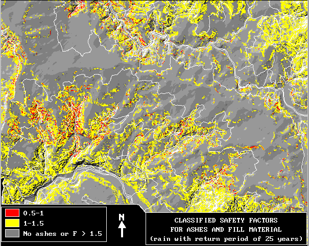
Figure 4: Classified safety-factor map for the study area calculated on the basis of groundwater levels related to a rainfall event with a return period of 20 years (scenario 2)
![]()
5. Failure probability maps
In the previous section, a method to calculate safety factors was explained, which uses average values for the various input parameters. Most of these factors contain a large degree of uncertainty. For this reason, the use of safety factors calculated from average values is not recommended. It is better to present the maps as average safety factors plus or minus the standard deviation. Standard deviations and variances can be calculated in two ways:
In this work a relatively simple formula for error propagation was used (equation [6]), based on Burrough (1987), which only takes into account the variance of the most important parameters (z, c´, tan n´).

where: VAR(F) = variance of the safety factor, VAR(c´) = variance of effective cohesion, VAR(tan n´) = variance of the tangent of the effective friction angle, VAR(z) = variance of the ash thickness, B1 and B2= two separate terms of equation [2].
The variances of the cohesion and the angle of internal friction for the ash deposits can be calculated from sampling point data. The standard deviations for ash deposits are in the order of 5 to 6 KPa for the cohesion, and 3 to 5° for the friction angle. The variances used here are: 25 KPa for c´ and 0.005 for tan(n´).
Determining the variance of ash thickness is much more difficult. From the field observations a very large variation of ash thickness for the same slope range was found. A simple calculation of standard deviations for each slope range would not yield satisfactory results. The approach that was chosen instead to determine the variance of ash thickness is based on the critical depth calculations, presented earlier in figure 3. Based on a variable groundwater table, and different seismic acceleration values, it is possible to draw approximate upper and lower curves for critical depths (see figure 5). In near horizontal slopes the variance will be the lowest. It will increase slightly in slope ranges of 5 to 15°, depending on the amount of erosion. Once the critical depth curve is reached, the difference between the maximum and minimum critical depth will become very large, depending on differences in groundwater depth/soil thickness ratios (m). In the steeper slope ranges the variance becomes small again as the maximum and minimum curves approach each other. It is assumed also that due to erosion there will be no more ash cover at slope angles larger than 60°.
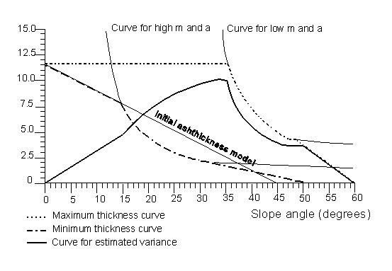
Figure 5: Method for deriving the variance of ash thickness. See text for explanation
In calculating the variance of the safety factor, only the variances of cohesion, friction angle and soil thickness were taken into account. The variance of the groundwater depth/soil depth ratio (m) as well as of the seismic acceleration were too difficult to take into account. Based on these, partly hypothetical, variances of the input factors, the variance map for the safety factor was calculated, using equation [6].
If it is assumed that the safety factors have a normal distribution, the deviation from the F=1 value can be calculated. This deviation is expressed by a Z-value (Blalock, 1979):

The Z-value can be considered as the distance between the average safety factor, AVG(F) which was calculated in the previous section, and the safety factor = 1, expressed in ordinates of Z-standard deviation. The total area under the normal curve is equal to 1. From a table of Z-values the area under the curve until the average safety factor can be obtained, which is equal to the probability that values lower than F=1 can occur. A graphical presentation is given in figure 6. The failure probability can be calculated for two different cases:
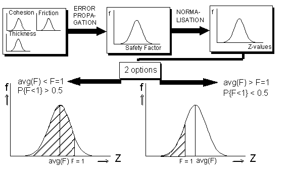
Figure 6: Schematic representation of the calculation of failure probability. See text for explanation
Probability maps were calculated for the six scenarios presented earlier on. Figure 7 shows the distribution of the resulting probability classes for the scenarios 2 and 5, with a differentiation of pixels with volcanic ashes and fill materials. It is clear from this figure that the pixels with fill materials, calculated from the differences in DTM's between 1949 and 1989, have the highest probability values.
The values for the failure probability calculated so far are only based upon the variance of the input parameters, cohesion, friction angle and soil thickness, given a certain magnitude for rainfall related groundwater and/or seismic acceleration. To derive at real probabilities, these values were multiplied with the probability that a given event, described in each of the scenarios, will occur within a given time period. In this case a design period of 20 years was used; the assumed design period for the low-budget housing projects in the Manizales area. The multiplication with the time probability will result in very low values for scenarios 3, 5 and 6. Scenario 3, fully saturated conditions, is a hypothetical one, and will therefore result in final probability values of 0. For scenarios 5 and 6 the final values will be very low, as the probability that both a rainfall event and an earthquake occur on the same day, will be low.
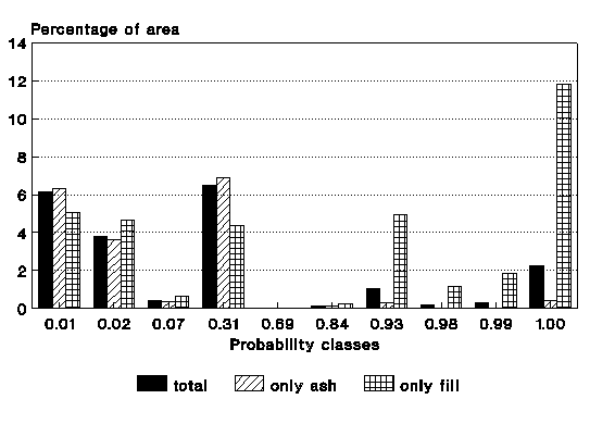
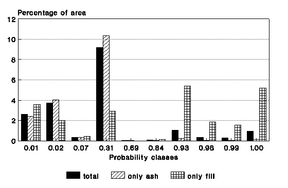
Figure 7: Classes for failure probability calculated using an infinite-slope model, calculated for two scenarios. Only probability values larger than 0 are displayed. Above: scenario 2. Below: scenario 5.
For the calculation of the overall hazard map for Manizales, all possible scenarios with respect to the magnitudes of the triggering factors should be calculated, and the results represented as probability values within a 20 year design period. Fortunately, a number of scenarios with combined rainfall and earthquake effects, can be neglected, as their time-probability will be so low that it will not be significant. Therefore, a selection was made of 15 scenarios, with the effect of one single triggering factor only. Out of the 15 maps produced for each of these scenarios, the highest probability value was selected for each pixel. This map shows values up to 1 in the steep squatter areas North and South of the city center. In those areas, it will be almost certain that a translational slide may occur within a 20 year period.
![]()
6. Discussion and conclusions
The final hazard map was checked with the occurrences of landslides. From the landslide distribution maps from the 1960's and 1980's, only the scarps of surficial translational landslides, that had occurred between 1960 and 1990, were selected. The resulting map was overlain with the hazard map. The result shows that 26.4 percent of the landslide scarps were in places with pixels, having a probability larger than 0.1. This is not a very good indication, as it is not required for a landslide to occur that all pixels within a potential landslide should should have high probability values. If the individual landslides are evaluated, 62% of the 438 landslides had pixels with a probability larger than 0.1. This means that 38 percent of the shallow translational landslides were not predicted. This may be caused by the fact that they did not occur in volcanic ashes, or that the landslide occurred within the ash deposits themselves, and not on the contact between ashes and residual soils, for which the hazard map is made.
To test the accuracy of the actual probability values, the hazard map was overlain with the total landslide distribution map of the 1980's. Of all pixels with a probability between 0.1 and 0.5, 20 percent was actually covered by landslides, and for the pixels with a probability larger than 0.5, only 26 percent. For this last group the expected value should be somewhere around 75 percent. This difference is caused mainly by the presence of fill materials on top of ashes, which have too high probability values (see figure 7). This leads to the conclusion that the resulting safety factors and probability values should not be used as absolute values. They are only indicative and can be used to test different scenarios of slip surfaces, groundwater depths, and seismic accelerations. They can also be used to analyze the sensitivity of the various input parameters.
The method presented here has a series of drawbacks, which should be taken into account:
The list of drawbacks makes clear that only general conclusions can be drawn from the resulting maps. The probability map for translational landslides should be used, in combination with landslide distribution maps and hazard maps for other landslide types, to make a general zonation map. The improvement of the resulting hazard map by collecting more data may be very difficult, as many variables are very heterogeneous within an urban area like Manizales. The method may be more applicable over more homogenous areas at a large scale (over 1:10.000).
![]()
Acknowledgements
The authors wish to thank the following persons for their valuable contribution: Niek Rengers, Rob Soeters, Jan Rupke, Theo van Asch, Jean Pierre Asté, Ofelia Tafur, Carlos Enrique Escobar, Henk Kruse, Juan B. Alzate, Dinand Alkema, Marnix Mosselman, Jose Luis Naranjo, Monica Dunoyer, Pradeep Mool, Achyuta Koirala, and Eric Mählman.
This work was financed by the European Union, UNESCO, the Netherlands Ministry for Education and Science and ITC.
References
Anderson, M.G. and Richards, K.S. (Eds) 1987. `Slope stability. Geotechnical engineering and Geomorphology'. Wiley & Sons, New York, 648 pp.
Blalock, H.M. 1979. `Social statistics', Mac Graw Hill, New York, 625 pp.
Brass, A., Wadge, G. and Reading, A.J. 1989. `Designing a Geographical Information System for the prediction of landsliding potential in the West Indies'. Proc. Economic Geology and Geotechnics of Active Tectonic Regions, University College, London, 3-7 April, 1989, 13 pp.
Burrough, P.A. 1986. `Principles of Geographical Information Systems for Land Resources Assessment'. Clarendon Press, Oxford, 194 pp.
Donovan, N.C. 1973. `A statistical evaluation of strong motion data including the February 9, 1971 San Fernando earthquake'. Proc. 5th World Conf. on Earthquake Engineering, Rome, Italy, Vol. 2, paper 155, 10 pp.
Geotecnia LTDA 1980. `Investigacion geotecnica postsismica del sector de la avenida Santander entre la Calles 47 y 48'. Unpublished report for the Corporacion Regional Autonoma de Manizales, Salamina y Aranzazu (CRAMSA), Manizales, Colombia, 30p.
Graham, J. 1984. `Methods of stability analysis'. In Brunsden, D. and Prior, D.B. (Eds), Slope Instability, Wiley & Sons, New York, 171-215.
Hammond, C.J., Prellwitz, R.W. and Miller, S.M. 1992. `Landslide hazard assessment using Monte Carlo simulation'. Proc. 6th Int. Symp. on Landslides, Christchurch, New Zealand, Vol. 2, 959-964.
Hansen, A. 1984. `Landslide Hazard Analysis'. In Brunsden, D. and Prior, D.B. (Eds), Slope Instability, Wiley & Sons, New York, 523-602.
Hays, W.N. 1980. `Procedures for estimating earthquake ground motions'. U.S. Geological Survey Professional Paper 1114, 77 pp.
Heuvelink, G.B.M. 1993. `Error propagation in quantitative spatial modelling'. Nederlandse Geografische Studies 163, University of Utrecht, 151 pp.
James, M.E. 1986. `Estudio sismotectonico en el area del viejo Caldas'. Internal report nr. 2008, Instituto de Geologia y Minas (INGEOMINAS), Medellin, Colombia, 113 pp.
Medvedev, A. 1965. `Engineering seismology'. National Technical Information Service (NTIS), TT 65- 50011, 260 pp.
Mulder, H.F.H.M. 1991. `Assessment of landslide hazard'. Nederlandse Geografische Studies, 124, University of Utrecht. 150p.
Murphy, W. and Vita-Finzi, C. 1991. `Landslides and seismicity: an application of remote sensing'. Proc. 8th Thematic Conf. on Geological Remote Sensing (ERIM), Denver, Colorado, USA, Vol. 2, 771-784.
Naranjo, J.L. and Rios, P.A. 1989. `Geologia de Manizales y sus alrededores y su influencia en los riesgos geologicos'. Revista Universidad de Caldas, Vol. 10 , 1-3, 113 pp. Universidad de Caldas, Manizales, Colombia.
Okimura, T. and Kawatani, T. 1986. `Mapping of the potential surface-failure sites on granite mountain slopes'. In Gardiner, J. (Ed), International Geomorphology, Part 1, John Wiley & Sons, 121-138.
Page, W. (Ed) 1986. `Geologia sismica y sismicidad del noroeste de Colombia'. Interconexion Electrica S.A., Medellin, 277p.
Terlien, M.T.J., Van Asch, Th.W.J, and Van Westen, C.J. in press. `Deterministic modelling in GIS-based landslide hazard assessment'. In: Advances in Natural and Technological Hazard Research. Kluwer.
Valencia, C.E. 1988. `Geotectonica regional del antiguo Caldas con enfasis en la aplicacion a la ingenieria sismica'. Unpublished MSc thesis, Universidad de los Andes, Bogotá, Colombia, 54 pp.
Van Asch, T.W.J, Van Westen, C.J., Blijenberg, H. and Terlien, M. 1992. `Quantitative landslide hazard analyses in volcanic ashes of the Chinchina area, Colombia'. Proc. 1er Simposio Int. sobre Sensores Remotes y Sistemas de Informacion Geografica para el estudio de Riesgos Naturales, Bogotá, Colombia, 10-12 march 1992, 433-443.
Van Asch, Th.W.J., Kuipers, B. and Van der Zanden,D.J. 1993. `An information system for large scale quantitative hazard analysis of landslides'. Z. Geomororph. N.F., Suppl.-Bd. 87, 133-140.
Van Westen C.J., Van Duren I., Kruse H.M.G., and Terlien M.T.J., 1993. `GISSIZ: training package for Geographic Information Systems in Slope Instability Zonation'. ITC-Publication Number 15, ITC, Enschede, The Netherlands. Vol. 1: Theory, 245 pp, Vol. 2: Exercises, 359 pp, 10 diskettes.
Van Westen, C.J., Rengers, N, Soeters, R. and Terlien, M.T.J. in press. `An engineering geological GIS data base for mountainous terrain'. Proc. 7th Cong. IAEG, Balkema.
Varnes, D.J. 1984. `Landslide Hazard Zonation: a review of principles and practice' UNESCO, Natural Hazards, No 3, 61 pp.
Ward, T.J., Ruh-Ming L. and Simons, D.B. 1982. `Mapping landslide hazards in forest watershed'. Journal of Geotechnical Engineering Division, Proceedings of the American Society of Civil Engineers, Vol 108, No. GT2, pp.319-324.